HD1970ElecEvol
Electronics Evolution

1970 Briefing Chart, one of many presented to Autonetics and TRW Guidance and Propulsion people brainstorming new concepts for an MX missile.
Sept 2003 I came across this figure when disposing of old papers. I emailed this to cousin Warren Kump stating this was done at the time CMOS first came out and that CMOS is what made it possible to make Microprocessors. Warren emailed back a show of interest – so I decided to write text to go with this chart. What follows shows why a fellow once said of me: ask you the time of day and you tell how to build a watch.
The Challenge
Our prior Post Boost Propulsion System work had come to an end, thus my Minuteman III System Requirements and Integration task ended. Our Autonetics division was not in the rocket engine system business, and my previous Flight Control Hydraulic systems work was at low ebb – I found myself well paid but without a job. Large numbers of people were being laid off and I was vulnerable to being one of them. I looked into what would be needed next. I figured there would be a follow on to Minuteman III and conversationally called it Missile X, which would indeed later be built as the MX missile. I reasoned that our Autonetics task would be to provide “hardened” electronics – as that was an unsolved problem at the close of Minuteman III. “Hardened” electronics was the name applied to improved survivability in a Nuclear blast environment. All of our Minuteman electronics, except for the Flight Control computer, was of the analog kind. It was obvious that performing in either ON or OFF mode would have better survivability than maintaining a quality linear signal after a blast. I went to my friends along “mahogany row”, some of whom I’d worked with since 1955, and suggested “someone” should start figuring how to convert our down stage analog nozzle control electronics to digital. They agreed with my reasoning. As I walked out, my friend Lou Purpura said, why don’t you look into that? I turned back and said, “but I don’t know anything about it, you know I’m a mechanical engineer.” Lou responded, “since when did that ever stop you?” He knew I’d created a variety of remote controls when operating an extreme temperature test lab for the Navaho program. This challenge created a need for me to know more about electronics.
I already had some knowledge of electronics from when I created remote controls for the Navaho & B-70 test program. I began work for North American Downey in 1955. At that time they were still using vacuum tubes for all missile electronics – however I listened as a few of the fellows told about new things called Transistors. I read a paper describing how they worked, telling of the flow of “holes” and “electrons” – it was very confusing how you’d make use of such a thing. But reset, it’s time for me to take you the reader back to a beginning.
A Story in Parts
I decided to tell this story in parts: 1923-1954 (radio), 1955-1969 (transistor), 1970-1980 (integrated circuits) & 1980-2000 (early PC). While recalling my electronics learning experiences, I was repeatedly reminded of how rapidly things changed. When reading Mark Twain’s Tom Sawyer and Huckleberry Finn I could relate to their adventures as I grew up in a time not far removed from theirs – when what you saw is what you got. Most people made the things they used or could see how they were made. No one tried to fathom how God’s creations worked. Seeds were planted and crops harvested, animals bred and raised – it happened. We human animals understand how a horse pulled a load, they were bigger and stronger.
When I began, shortly after WW I, wheat was hauled to town by teams of horses. My father, born in a homestead sod house, drove an early vintage Model-T as field man for a Loan and Abstract company. My grandfather, who died the week I was born, grew up in Illinois while the army was chasing Indians and others extended railroad tracks west. Dad replaced our kerosene lamps with light bulbs dangling from cords, they used electricity from the towns new power plant. In the stillness of the night we could hear sounds – dad said that was the sound of the power plants diesel engines making electricity. Before starting school dad shared his earphones so I could hear sounds come out of a wooden box – fiddling with an antenna which somehow was the source of sound. Dad called the box a radio. About a year later we had a radio of our own, with a large round speaker on top of a big metal box.
The world was full of amazing things, like sun up, sun down. A moon that changed shape, stars that slowly moved, water falling out of the sky. I was told of people with yellow skin and slanted eyes, who stood upside down on the other side of our earth – earth being the dirt beneath my feet – and they did not fall off! So what was so strange about sound coming over a wire exposed to the air.
It was my privilege to be permitted to move about a near by milling company and watch workmen before old enough to start school. It was there I watched them start a large one cylinder engine that turned a huge flywheel that was connected with a flat belt to line shafting that extended through out the mill to power milling machines. I could readily understand what I could see. I also watched as workmen hoisted an electric motor, listening as they said this was the new and better way to power the machines. I saw abandon big steam tractors, replaced by tractors with gasoline engines – and now electric motors were replacing gasoline engines. It was obvious trucks would soon replace horses for hauling wheat to the mill.
Electricity was now running moms washing machine – in addition to lighting bulbs and having something to do with making the radio work. The world was full of things I didn’t understand, but there were some like man made things – knowable things. These were fascinating – I wanted to know how they worked?
The world I experienced is now gone, kids of today learn from TV, they quickly adapt to computers, and enjoy the magic of cell phones and the internet. These are like the air they breath, as if they had always been. I’m sure they too enjoy the thrill of learning, the curious always want to know how things work. Today even things made by God are within range of comprehension. Most of us use complex things without a clue as to how they work or are made. Technology evolves, building on itself, creating ever more complex things. I can only guess the future, of things to come. But I can share with you my learning experience as a participant in this never ending process.
1923-1954 Radio
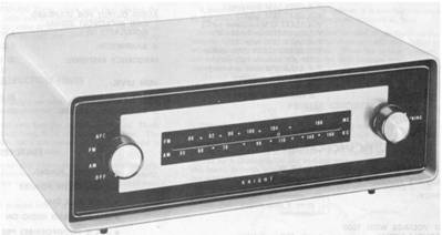
The first radio’s in our home town (Oberlin KS) arrived about 1923, the same time I did. Dad borrowed one from a friend. It was a wood box, with a dial, an antenna wire and a place to plug in ear phones. I’d watch dad as he slowly turned the dial hearing whistles escaping the ear phones as he searched. There was only one good station, KMMJ in Topeka. I knew he’d found it when his face lit up – it was then he’d let me listen – we shared the earphones. The sound would fade causing more hunting with the dial. After a time dad said the batteries gone dead – I’ll need to get a new battery when I take it back. About 1927 my parents bought an Atwater Kent radio, with an 15” speaker atop a 7”x 12” x 20” steel case. No tube had a number greater than 10. Farm radios used A and B batteries. If lived in town you could plug into electricity and didn’t need an A battery to heat tubes. But you needed the B battery that operated the tubes. The B battery cost more as it was made of many small 1.5 V batteries connected in series to output a high voltage.


When in high school my folks bought me a radio, similar to the one shown. It was a mass produced standard of the day. The tube filaments were connected in series, heated by wall plug AC power. The first number on the tube states it’s voltage drop. Like 35Z5, 12SA7, 12SK7, 12SQ7, 50L6 for a total of 110 volts. The 35Z5 is a rectifier tube, converting AC to DC and is followed by resistor, capacitor, and coil (choke) filters to smooth out the ripples. The antenna, upper left, is connected to a “signal selector” called a “tank circuit” consisting of a variable capacitor and fixed inductor coil in parallel. The capacitor—inductor combination capture only one frequency, which they “bounces” between them, as if holding the selected “tuned” signal in a tank – all other frequencies pass through and are not “held”. When the operator “tunes in” he is rotating the variable capacitor, a gang of aluminum disks. The 12SA7 is an oscillator-mixer-amplifier tube. The oscillator part generates a “carrier” frequency then mixes the selected input signal with it, in this case causing AM (amplitude modulation) of the carrier signal. The 12SA7 and 12SK7 amplify the AM signal, passing it to the next tube through IF (intermediate frequency transformers). These are the large cans in the above right photo. The 12SQ7 tube detects and separates the amplified radio signal from the carrier signal and applies it to the 50L6 power output tube which drives the speaker.


The
above radio used AC power direct, without a transformer, the 35Z5 tube served
as a diode (flow in one direction only), producing half-wave rectification.
I took my radio with me when I went into service. I packed it in my barracks bag and when removed found the plastic case crushed. I had a wooded case made and took it overseas with me. It worked for a while then abruptly quite? I asked radio and radar officers in our quarters what might be wrong – they shrugged saying it might be anything. By the time they returned from watching a movie I had it playing. Surprised, they asked what I’d done to fix it? I said I don’t know?
I connected it to a permanent magnet speaker I’d found. That worked but was very noisy so I reconnected the big speaker coil in series as it had been – then it worked just fine. They said oh yes, your small speaker coil went out and the new permanent magnet speaker fixed that. The noise was because you removed the choke filter from the power supply. Your speaker used an electro magnet, rather than a permanent magnet – that coil did double duty as a choke to filter DC power.


When being shipped from FL to CA while in service I bought a book on radio and read it on the train. It was a bit much to absorb in a short time but it permitted an acquaintance with the principles and terms. Only later did I appreciate what was being expressed: 1)Carrier waves lifted tiny signals up out of the mud. 2) IF transformers separated amplification stages. To appreciate this you need to understand how a vacuum tube works.

A vacuum tube operates on DC voltage. A heated cathode “boils” off electrons into the evacuated tube space. The cathode is connected to signal ground and the plate to high (+) DC voltage to attract negative (-) charged electrons. Between these is the screen grid, a signal applied to the grid aids or hinders the flow of electrons to the plate. A grid must be adjusted, “biased”, to a DC voltage level, between that of the cathode and plate by an amount which permits a varying input signal to be amplified to a larger signal and retain it’s full wave form, without being clipped off. The tube’s amplification is not perfectly linear. By use of a carrier signal, a tiny signal can be lifted out of the “mud” near ground and placed in the linear region for amplification. I didn’t really appreciate the meaning of “bias” and how this worked until adjusting bias for transistor amplification.

AM vs FM radio
AM (amplitude modulation) was used on all early radios. FM (frequency modulation) came out later, with FM a tube biased was optimized to handle one amplitude only, the objective, to achieve better fidelity.
Fritz Gardner a friend of mine was assigned from Signal Corp to Air Corp in early WW II. As a graduate electrical engineer he was able to solve the B-17 turbo supercharger controller problem. The designer forgot to install grid bias resistors for the amplifier tubes! They were cherry picking tubes that happened to work – for a while.
DC separation of amplifier stages is achieved by use of IF transformers. The amplified signal, “sucked” to a high DC voltage plate is applied to the input winding of the isolating transformer. The signal is electro-magnetically passed, with no wiring connection, to the output winding and applied as a pre amplified signal on top of the DC bias of the next tube. It’s a terrific stunt where tubes work in parallel boosting the signal.
My first hands on Radio work was installing an old but functional car radio in my Model-T, it was the only Model-T in the county equipped with a radio.
From the time DeForrest invented the amplifying tube in 1906, it required much innovation, by many, on how to apply them. By WW I radio was playing it’s roll communicating over long distances using short wave. By WW II it was a highly refined art.
Navaho 1955-1958
I was in charge of an extreme temperature test facility in Downey CA where it was necessary to instrument and remotely control flight control equipment. During this time Bob Kelley, an excellent electrical engineer without a degree, helped me understand more about electronics and the new transistor. He told of how I could make a HiFi Amplifier without the use of the big transformers used in vacuum tube amplifiers to drive speakers. This led to numerous experiments with transistor kits which resulted in building my own “electronics work bench”. I built a “home grown” variable power supply plus Oscilloscope, Vacuum Tube Voltmeter and Signal Generator from Kits -- plus other home made supportive devices. This experience was very valuable. I applied what I learned at home to work and visa versa.
I read parts catalogs to learn the names and symbols used, so I could understand what the electronics engineers coming to our facility were talking about. My previous experience as Airplane Mechanic, Civil Engineer and Process Engineer on tooling to build airframes did not help. Much of the changing domain was new to me.


Names of the players


Making a power supply was one of the first priorities when experimenting with electronics. The first ones were “dedicated” fixed transformer power supplies delivering the voltage needed.
Variable Power Supplies
Variac (Auto-transformer)
I made a variable power supplies by use of a Variac Transformer (sometimes called Auto transformer) followed by rectifier diodes and filtering capacitors. Control of the output was later refined by use of transistor filtering as shown above right.
Silicon
Controlled Rectifiers.
Silicon Controlled Rectifiers (SCR) had come out, where an incoming alternating current could be clipped, controlling what portion was passed. For the first time AC voltage could be “stepped down” without the need of a transformer. Light dimming devices for the home used this method. Using information from various catalogs, I made my own variable power supply as shown in the following figure. It worked quite well and was built into my work bench power supply. SCRs were not used on our missile program as they were considered too vulnerable to external influences.

Silicon Controlled Rectifier Variable Power Supply built during MM II.

My first electronic projects were simple kits, such as making a radio inside a Skippy Peanut jar. These increased to bigger and bigger kits of all kinds. Our kids were little and I built a kitchen cabinet table and phonograph cabinet, including the phono kit inside.

Knight Kit AM-FM Tuner Knight Kit Wireless Broadcaster

Kit making led to building a complete HiFi Setup including a cabinet. A tape recorder was in the upper left pull out drawer. A hifi phonograph player in the upper right pull out drawer. The hifi tuner and hifi amplifier were in the upper middle section with dual speaker systems on each side and a center section for holding supplies. The cabinet was made from one sheet of walnut – after much preplanning so the grain patterns would match. The lid lifted up for access to parts.

This vacuum tube Heath Kit HiFi Amplifier is typical of what fellows were building at the time, I built one. It played well but was very heavy and got very hot.

All Transistor HiFi Amplifier used in the above cabinet for years until the kids twisted the wires behind the knob loose at a time I was too busy to fix it. It was superior to the vacuum tube kit.
Thanks to advice from Bob Kelley I was able to make the above HiFi Sterio Amplifier. This used early transistors and was the incentive for building test equipment from kits. Each amplifier stage was fine tuned by use of signal generator, oscilloscope and Vacuum Tube Voltmeter. (I learned the value of a Vacuum Tube Voltmeter, as compared to a standard Volt-Ohm Meter, when asked to align position transducers on the Navaho G-26 Booster. A vacuum tube voltmeter could read a small signal and be isolated from the signal being read, a Volt-Ohm meter could not.) With these instruments I could bias each amplifier stage to operate in a linear region. I used square wave to do this alignment – Kelly said if it’s good using square wave it will work for any frequency. I demonstrate the alignment quality to my father when he was here – he smiled approvingly while shaking his head, not understanding. This HiFi Amplifier is now in the Oberlin KS museum.
Another endeavor was to build a transistor radio. My first attempt failed, I was very discouraged, A year later, driven by tenacity to not admit defeat, I found the IF coils were not wired as shown on the diagram, when I removed the cases and check continuity. I wired according to their real connections and it worked!! This was built before small “Japanese” transistor radios swept the marketplace.
Minuteman I, 1959-1962 Discrete Semi Conductor Parts
Eliot Buxton, our assistant chief engineer, convinced decision makers our flight control computer should be digital and use transistors – and that our down stage analog servo controls electronic should be made with transistors. The main reason for this was to survive 14 g’s acceleration of solid propellant engines coming out of a silo. No aircraft or other missile was subjected to this level of acceleration or severe vibration. So it came to be that vacuum tube circuits were rebuilt using transistors rather than tubes. Minuteman I electronics consisted of transistors, and associated parts, placed on pre-wired circuit cards. New IBM computers were also built this way.


People knew digital electronics was the coming thing and attempts were made to come up with digital valves and digital actuators. The above left photo shows an experimental digital valve. It was believed you could not command analog servo valves, as above right, with digital electronics. One company designed and built a segmented actuator where each segment could be commanded by a binary bit in accordance with the size of that bit.
The electronically commanded hydraulic servo valve was a new invention, used for the first time on the Navaho missile. By the time of MM I production high quality servo valves had evolved similar to the one shown above right. A vacuum tube driver commanded an 8 ma coil which moved a flapper which ported fluid to proportionally move a spool that ported high pressure hydraulic fluid to a actuator. These were small, fast acting and reliable. The Minuteman valves used dry torque motors developed by MOOG, prior wet coils attracted contaminates. When I took on the challenge in 1970 I had no idea of how to command these analog valves from a digital error command – many capable people said it couldn’t be done.

Logic devices were built on cards
using combinations of resistors, diodes and transistors for each function.

Minuteman I electronics was made up of discrete parts on removable cards behind the warhead, accessible from the side of the missile. All except the Flight Control Computer were analog circuits. I knew nothing of this electronics at the time. I’m sure the digital computer used AND & NAND, OR & NOR, EXOR & EXNOR logic made of discrete parts from which they made functional elements such as shift registers, bit adders, counters and storage registers. Boolean Algebra was used to help determine how to use these devices in a most efficient way.
Operational Amplifiers – a Primary Analog Computers building block
Use of carrier frequencies to accurately “carry”
small signals
Art Greer came to me and said they had no idea what the loads would be for tilting nozzles. He was aware of the unexpected problems encountered with the Hound Dog missile control and wanted to be prepared for the unforeseen. Paris Stafford and I had often discussed our method of creating an actuator load, for high temperature seal tests; our steady pressure relief valve method did not represent what the actuator would actually see.
Most of the controls analysis fellows had been taking after work classes, using the text book Control Systems Synthesis by Truxel. These analytical methods were not taught when I was in school. I bought a book on servo controls by Savant and studied it on my own – so I could at least understand what they were talking about. Joe Cherney, who worked on the MM I Digital Computer, told me servo control theory began with fire control systems in WW II; he had worked on those and the method was kept secret. Walt Evans one of the Inertial Navigation engineers during the Navaho program came up with the “Root Locus” (1948) method of determining if a servo loop was stable.
Simulations were made, using analog computers, applying methods called controls synthesis and a mathematics called Laplace Transforms. When I was in school we were taught the use of differential equations which was performed using Differential Calculus, we did not learn of Laplace unless you were a math major. Laplace would be superceded by Z-Transforms and all of that by Sample Data when digital computers took over from analog computers.
Art and I talked about the kinds of loads such as: Coulomb friction, Spring a function of position, those a function of velocity, and those a function of acceleration. In differential equation terminology these were expressed as: Load = Kf (friction) + Ks*x (distance spring) + Kv*dx/dt (velocity) + Ka*dx/dt(dx/dt) (acceleration). Where Kf, Ks, Kv, Ka are mathematical coefficient (values) for each term. Where x is distance, dx/dt the rate of change in distance, dx/dt(dx/dt) the rate of change in velocity To simplify notations, x with dot above, was used as short hand for dx/dt. A single dot for the first and a double dot for the second derivative. [In college I had trouble with terminologies. To me the differential was the gears in the rear axle of a car, and I’d never heard of an increment. I finally grasped that dx/dt expressed the difference in position vs time.]
Art said I should come up with a means of “programming” a load cylinder to simulate various kinds of loads -- and to provide a general purpose set of resistors and capacitors with which to create shaping networks to compensate for loads we might encounter. I talked it over with Paris Stafford who said go ahead, see what you can come up with.
We had test fixtures on which we could place a Minuteman actuator and operate it against a load cylinder. (You could watch those small actuators bend heavy steel plate.) With this beginning, I connected the load cylinder to a “pressure control servo valve” and rigged it to change pressure as a function of position. But I had difficulty finding velocity and accelerometer sensors. One of the fellows said you can convert the rate of change in position to be velocity and the rate of change in velocity to be acceleration – they do that in the simulation lab using analog computers.
I talked it over with Stafford who said fine, but you’re going to be very busy, don’t try to build this yourself. Define what you want and we’ll buy it. (He didn’t say so but probably knew they were moving Art to Project office and me to lead engineer for hydraulic controls.)
I defined what we wanted, and purchasing sent it out to those who make simulation lab analog computers . I spent an day talking with the supplier, and was very impressed -- he immediately knew what we wanted and how to do it. At my request he left a Philbrick Operational Amplifiers catalog, the main ingredient of his solution. He was given the go ahead and I read about Operational Amplifiers. The “load simulator” had became an analog computer commanded test fixture.
Operational Amplifiers are used to simulate systems by shaping signals to represent real world dynamic conditions. Operational Amplifiers used choppers to create a carrier frequency. Small signals are superimposed on the “carrier” then “detected” after “shaping”. This lifts small signals out of the mud near ground and puts them in the linear region of a vacuum tube amplifier. (I recognized the principle as similar to radio). The operational amplifiers chopper was like a radio’s oscillator and car radios vibrator – different names for similar function. I had learned much from this – but nothing of much help for the pending digital effort. (Henry Ford equipped Model-T’s with four dedicated “coils” designed to serve as vibrators to generate high voltage from battery power. Making and breaking contacts created AC voltage applied to encased coils of tin foil which generated high voltage applied to spark plugs.)
Minuteman II 1962-1964 -- The first Integrated Circuits
Minuteman II used newly developed “integrated” circuits. These were special made “flat-packs”. The following image is of an analog amplifier. There were many MM parts, such as flip flops and logic devices in similar packages. At the time I knew nothing of what was in these packages or how they worked.

Minuteman II analog integrated circuit used
for our Freon dump system,
photo from paper I gave in KC MO for society of automotive engineers
aircraft controls section.
Minuteman III 1965-1969 – Highly Reliable Family of Integrated Circuits
Minuteman III used even newer integrated circuits. There was a family of “Minuteman Parts” made in tightly controlled clean room facilities. This resulted in a tremendous increase in reliability. Previously “flakes” of contaminate would come loose, especially under sever vibration, causing failure. The electronics industry soon aware they could get more good chips (better yield) from super clean facilities began using cleaner methods for commercial parts. Reliability of all electronics improved dramatically. This special Minuteman Reliability money was to make it possible to later build microprocessors.

Minuteman III Guidance & Control section
MM III integrated circuits permitted packing much electronics in smaller packages. The above shows the Inertial Navigation computer, Flight Control computer and Flight Control interface electronics.
Logic
devices and their Truth Tables
As I began learning about digital electronics I felt I was chasing a departed train. However I had an advantage, the new digital devices were so new, most of the electronics engineers still engrossed with analog didn’t know them. The commercial world was now producing integrated circuits – the digital world was catching on and I was there to sample the new devices. I had to master logic devices as these were the building blocks for other devices. There were AND & NAND, OR & NOR, EXOR & EXNOR “logic devices”, Inverters and Flip-Flops. I memorized truth tables, names of the devices and associated terminology.
 .
.
Logic devices, the building blocks
Inverters, though not a logic devices but are used extensively; the output is the inverse of the input.


The commercial world was building logic functions in sets of four in standard packages. Trade magazines advertised new devices and I sent for more information. Excellent material was available for the asking.

on or off output using a transistor
I had to know how a transistor worked to perform logic. The above shows a transistor in series with a resistor. Transistor parts are: collector, emitter and base. The junction of these can be made with P or N “seasoned” material. For P material electrons flow from emitter to base, and for N material electrons flow from base to emitter; an arrow is shown to indicate current flow, the above example is for an N transistor. Thus a user has options on how to connect parts. The above is the typical arrangement for defining an output; with a “pull up” resistor or “pull down transistor. To turn the transistor ON the base must be “sourced” with a current, when “on” the above out terminal is pulled to ground, when off the output is pulled hi, in this case 5 Vdc. The upper resistor can be likened to a spring, the out is always up unless pulled down.

How
to command transistors
A friend of mine, Emil Kohler, taught me how to “think” when connecting transistors – you “source” or “sink” the base for on-off control – this avoided thinking of “holes” and “electron” flow. The phenomenon had been described by Physicists but technicians connect the real world. I learned the hard way that diodes are marked for “conventional flow” where as electrons flow upstream into rather than out of the arrow – they are wired as like a car battery plus to minus, though electrons flow minus to plus.
The need for inductive kick back protection.
If a coil, such as on a solenoid valve, is connected in series with a transistor, the solenoid can be activated by turning the a power transistor on. Such an application enters another domain, that of inductive “kick back” (a misnomer) where current flowing through a coil builds a flux field, then when current flow is cut by an open switch, the collapsing field tries to push current through the OFF switch. Minuteman was one of the first to use transistors for such an application. The induced voltage far exceeded what the transistor switch could handle. We had to install “kick back” diodes and flow limiting resistors in parallel with the coil to provide a path to carry the induced current back to the power source and thus protect the transistor switch. Power transistors can now be purchased with these diodes built in. (Inductive “kick back” is what caused points, on pre 1965 car distributors, to pit and burn out -- when the points broke, the induced high voltage would jump the gap – semiconductors solved that problem and people no longer have to repeatedly replace and reset points.)


The logic devices were combine to make a Flip-Flop. The Output O is changed to a Q to distinguish it from a Zero. If output Q is 1 then Q with a line above, called “notQ”, is the inverse of Q. A “1” (high) “set” command causes the Q to be “1” and notQ to be “0” (low). A “1” “reset” command causes Q to become “0” and notQ to be “1”. A “clocked” flip flop does not implement a signal applied to Set or Reset, until a “1” is applied to the clock pin. This is a powerful building block and one of the first “integrated circuits widely used and sometimes specified as “J K Flip Flops”, a more refined version to preclude ambiguity.


Counters, Shift Registers & Storage Registers (Latches) were some of the first items assembled using flip-flop building blocks.

From the beginning I knew I’d need a clock to time events. The only clock diagrams I could find were crystal timed clocks derived from vacuum tube circuits. I was delighted to find an article which showed how to make a clock using logic elements, a capacitor and two resistors. These worked fantastically well. With these I could run a binary counter. A binary counter output could be expressed as bit steps by use of a 1 of 16 decoder chip. Using variations of these methods I could define any increment of time in a system of parts. Applied data could be clocked (or strobed) into a register and held steady until read as input to another device at a later time increment. I created a timing diagrams to control operation the system of parts.

TTL came out about 1969, I learned about it from full page adds by multiple suppliers. I sent off for their literature which was very instructive. They were advertising new 4 bit sets of logic, holding registers, shift registers and counters – initially there were no arithmetic devices. This literature convinced me it should be possible to control the down stage servos using digital devices. I focused on how to apply these devices TTL sweep the industry – until replaced by CMOS.
My First Digital System
My initial concept was to replace analog servo controls with digital servo controls in each of the three downstage nozzle control units – and communicate using a four wire “data buss”: +5 Vdc, signal ground, data and clock inside a shielded cable.


Minuteman Raceway and electrical cable within to be replaced
Missile Data Bus
The few data bus wires supported the idea of removing the protruding raceways on the side of the missile. Minuteman raceway conduits were six inches high. They caught winds when coming out of a silo making it necessary to provide robust roll control authority. I fashioned my communication bus after a rural telephone line – where each party used the same line, each having their own “ring” code.
The digital data bus was the simplest part of the system to design. Due to my ignorance I didn’t know protocols had been evolved to do such things – so I designed my own. I used a clock to shift data from a send shift register to a receiving shift register and load or unloaded their content in adjacent storage registers. I defined command and feedback messages with addresses for who to and who from. I used newly available 4 bit TTL chips to do this. Later UART (Universal Asynchronous Receiver Transmitter) chips, as in today’s desk top computers, were designed to perform such tasks.
Numbering convention

I soon learned that in the digital electronics world numbering often started at zero: 1 to 16 was often expressed as 0 to 15. I was also caused to think and covert between Decimal, Binary & Hexadecimal. Hexadecimal permitted showing a “nibble” (four bits) in one column, and thus a “byte” (eight bits) in two columns. [Vern Chandler chairman of our 19th Bomb Group Association at the time got after me for using 0 as if it was a “count” rather than representing nothing. I responded that it’s a matter of what world you live in.] ASCII (American Standard Code version II) the alpha numeric code used by computers, had it’s origin in telegraph, and requires 7 bits to define a numbers and letters with the 8th bit serving special functions. Early on it became important to understand these terms.
Up-Down Counter as Summing Junction
The digital servo loop was more difficult, the task was to compare the position command with position feedback to determine the amount of error – then command the control valve to correct the error. This is simple task for an analog system where commands and feedback meet at a “summing junction” between two resistors, where feedback is negatively connected to cancel a command. One day driving to work I had trouble with my odometer cable – this triggered the idea that an odometer could be caused to count up or down. That gave birth to the idea of using an up-down counter to serve as a summing junction. A command would inserted then and down counted by the feedback to determine the errort.


I planned to parallel load the incoming binary command into an up-down counter, then down counted the feedback according to the sign bit and read the output error as the valve command. I didn’t need to do arithmetic.
But how was I to convert square wave feedback to clock the counter?
Feedback signal

Position Transducer body and slug

Our position transducers were slug coupled transformers with canceling outputs at null and plus one direction and minus the other. They were excited at about 5khz with chopped DC which resulted in a square wave output. The output was converted to DC by use of a full wave demodulator.

Demodulator is like a full bridge rectifier except the diodes are replaced with transistors. Diodes have a voltage threshold that voids null (near zero) level signals. My later design used CMOS transmission gates for the demodulator switches, driven by transducer excitation signal. Position was now expressed as plus or minus dc amplitude and used a level detector to determine sign (up or down).
Voltage to Frequency Conversion
 Motorola
had come out with a voltage controlled multivibrator chip. I applied the feedback dc voltage magnitude
to the multivibrator and applied this frequency representation of position
magnitude to the up/down counter in accordance with the sign bit such that
feedback was subtracting from the preloaded binary command. The feedback frequency and duration of the
count were calibrated to have the same binary scale as the command. I knew this was a make do method, but it was
a way to get started. (I would later
submit and be issued a patent for a digital feedback method. I was requested to submit the idea for
patent even though I had abandon the concept.)
Motorola
had come out with a voltage controlled multivibrator chip. I applied the feedback dc voltage magnitude
to the multivibrator and applied this frequency representation of position
magnitude to the up/down counter in accordance with the sign bit such that
feedback was subtracting from the preloaded binary command. The feedback frequency and duration of the
count were calibrated to have the same binary scale as the command. I knew this was a make do method, but it was
a way to get started. (I would later
submit and be issued a patent for a digital feedback method. I was requested to submit the idea for
patent even though I had abandon the concept.)
Servo Command Generator
I simulated an upstage computer signal the same way, using pitch and yaw variable resistors to provide voltage inputs to pitch and yaw multi-vibrators. An up stage command “joy stick” could command an equivalent down stage nozzle movement. I built the aluminum tube joy stick with pitch and yaw variable potentiometer in my shop at home.
After Work Classes by Microelectronics Division Chief Engineer
I attended after work classes taught by Microelectronic chief engineer. These were excellent providing insight on how the new family of MOS (Metal Oxide Semiconductor) devices worked. We were given tours of their on site facilities where they were making Silicon on Saphire high density read only memory chips, and would later make 6502 micro processor chips. They had a number of company and government sponsored endeavors going, all of which used MOS devices – of the N or P kind. This first figure in this document shows how N type silicon glass could be masked, and etched to create “pockets” in N material into which P material could be deposited. Transistors built in layers were interconnected with aluminum deposited as the top layer. Tiny wires would then be connected to carry these connections out to packaged pins permitting connection to the real world of a circuit board. The terminals of a transistor are Source Drain and Gate. A voltage applied to a gate caused the transistor to turn on or off by field effect – no current flows from command to output! This fascinated me, conventional bipolar transistor commands flow connect to the output – the command mixes with the output.

Out of this came the concept of CMOS (Complimentary MOS) where a P device was connected in series with an N device. If for example the P device was commanded ON the N device is commanded OFF – and the reverse if the command was reversed. The devices compliment each other. The highly significant attribute of this is that there was no power is consumed when held in a steady state. Current flows only when the devices changed state, a very fast change, when being clocked by a change in logic – which applies to only some of the transistors at a given time. This low power consumption and the ability to make thousands of these on a given chip made the microprocessor possible. However I’m ahead of my story.

I was further fascinated by what was shown in RCA and Motorola information as a Transmission Gate. A P-MOS connected in parallel with a N-MOS will can be commanded to both on or both off causing them to be an analog switch. The ON command to a P, if inverted and applied to the N will turn both on, conversely both off. RCA supplied a chip with four transmission gates (analog signal gates). I sent for samples of this new chip and used it demodulate the position transducers square wave output to dc output.

Four transistor H switch Servo Valve Driver
Transistors only heat when throttling
current
It was very importance was to find a way to command an analog servo valve. When visiting with Emil Kohler he said why don’t you use an H switch? I asked, what’s that? He said think of it like a football goal post where the valve coil is the horizontal bar. You put a switch in each leg. Assume the top is plus and the bottom ground – turn on upper left and lower right switches and you cause current to flow left to right through the coil. Reverse the switches and current flows right to left. That was it, so simple! The new CMOS chip with four independent transmission gates seemed ideal – if this tiny device could pass 8 ma of current – these were logic level signal switches not drivers though the current was low. The switch would either be full on or full off. Transistors do not heat when full on, or full off, they only heat when throttling current flow by acting as a variable resistor. All analog valve switches throttled current to control flow rate and would heat. I rigged a test set up in the lab – it worked beautifully!! The chip did not heat when cycled on–off. I hurried to show those who had told me you could not command an analog valve with a digital chip.

Combination of parts to drive the servo valve.
How to convert a binary
number to a valve command.
I recalled testing Johns Hopkins University’s “Accelerating Switching Valve”, they dithered the spool to clear contaminates. I recalled how Bob Kelley had ignored noise on a servo valve signal saying the valve cannot respond to high frequencies, it averages the noise. The valve coil is an integrator. This brought me to the idea of converting a binary error signal to a % on time, where lesser commands are a % of full on. By rapidly applying partial commands the servo valve would integrate (average) them. I decided to use an error ramp of 0 to 16 bits, 16 bits being full on. I made a 16 bit shift register and clock the shift register at feedback excitation frequency. All 0’s were 100 % off and all 1’s were 100 % on with 16 steps in between. The sign bit determined witch pair of switches were commanded. It worked beautifully!! I had a dickens of a time using logic to convert a binary number to a % on time, a 1 for every error bit. I solved the problem by using a look up table. Some called it pulse width modulation. This part worked beautifully.
System built and Demonstrated
This system was build and demonstrated. Tom Shuler, head of Autonetics at the time came by to see what had been done. I demonstrated how it worked by moving the Joy sticks – then stepped back so he could try it out. We watched his face brighten with a smile when observing actuators at the bottom of the electronic console track his wiggling the “joy stick” at the top -- aware the only connection was four small wires. We had connected two P-106 Post Boost axial engine electrical actuators to a plastic funnel to simulate thrust vector control of a rocket nozzle.
Need 7th order filtering
It worked, but not well enough. The AF was sponsoring efforts for motor contractors to develop nozzle control systems for newly invented movable nozzles built into a solid propellant case. The TRW stipulated with AF approval, that they could not use hydraulics actuators. The reason given that it was already known how to do that. We anticipated these new kinds of servos, powered by 100 hp solid propellant gas generators would require 7th order filtering to tame them. This would require the use of a signal processor capable of perform fast multiplies by repeated addition. This was a totally new ball game. Since the new nozzle designs were built into the motor case, the AF decided, on TRW recommendation, to transfer nozzle servo controls to the motor contractors. With Autonetics out of the nozzle control business I did a 180 change in concept – I moved the servo controls electronics up stage, for time shared processing and hard wired signals to and from down stage valves and position transducers. This still permitted a flat raceway. By this time a four bit TTL Arithmetic Logic chip had come out along with a Look Ahead Carry chip. Using these I was able to make an 8 bit signal processor that could be time shared for four servos at the same time, two for the stage to be terminated and two for the new stage being activated. This required a different set of coefficients for each of four stages.

Blair Bona’s Rosetta Stone and Sample Data Filter
Sample Data Systems
I agonized over how to process “filters” or shaping networks as they were called in the analog world. Dr Blair Bona who would often came by and chat with Malcom Johnson, my office mate, and I observed I was reading books on servo control theory. He’d ask what book I was reading, and comment on what he thought of the book. I was unaware he’d written and published a book on how to do this kind of thing. He would later call me in his office and show me a book his publisher had sent for review – it was written in Japanese – except for the mathematical terms.
Aware of what I was trying to do, he said here, let me help you – can I erase this stuff on your black board? I said sure. He then wrote what to me was the Rosetta Stone translation between Differential Equations, Laplace Transforms, Z Transforms and the Sample Data equivalent. The following figure is derived from what he wrote on the board. This was fantastic, now I knew exactly what I had to do – what the arithmetic unit had to do. But my enthusiasm was short lived – doing digital arithmetic was not all that simple.
The Second System – Include A Signal
Processor to do Arithmetic
Digital
Arithmetic
1’s or 2’s compliment numbers, Arithmetic Logic, look
ahead carry and Booths algorithm
While shopping in south coast plaza I came across a book on Digital Computing – bought it and read and read trying to comprehend the process. To do digital arithmetic you must convert binary numbers to either 1’s compliment of 2’s compliment form.
This began the process of trying figure out how to connect 4 bit ALU (Arithmetic Logic Unit) chips and Look Ahead Carry chips to do 8 bit parallel additions to complete 8 bit multiply calculations. A first step was fully understanding the ALU chip, as shown in the following figure.


1’s & 2’s Compliment Numbering systems Arithmetic Algorithm for 2’s compliment
Though clearly defined, it was difficult for me to understand how to handle 1’s ir 2’s complement numbers – until I came across the expression of an algorithm to accomplish that. Since ALU chips were newly available most text books only described serial “bit adders” where shift registers cycled bits to multiply bytes of data. I had the advantage of a parallel adder.
At the time I was completely unaware I was designing a digital computer – to me it was a dedicated signal processor for a given stage. Only later did the concept change to a time shared processor, located up stage rather than down stage. Time sharing and the use of different coefficients for each stage caused it to become a programmable computer. Being ignorant of what I was getting into, I blundered my way ahead.
I’ll not drag you the reader through the architectural agony I went through in making the system work. The following diagrams are a fraction of the many I put together in the process of first creating a dedicated processor for a pair of servo actuators to that of handling four sets of such servos with two sets at a given time.

Open Collector method for Single data bus from multiple registers

Open Collector Electronics
This diagram reminds me of the problem of applying data from several registers through a common data buss, like to an Arithmetic Unit. For early TTL devices this was done by using an “open collector” with common pull up resistors. The figure show standard and open collector TTL gates. A data bus line was always hi unless pulled low. This would later be solved by use of Tri-State Logic.
Tri-State Electronics
Tri-State logic that followed was either hi or low or open. This was achieved in CMOS by use of transmission gates. Remember CMOS uses field effect for control of a Transmission Gate device the command is isolated from data. When not commanded low or hi it is open.
Tri-State for Aircraft
Later when working on a C-130 Gunship & C-17 Cargo plane programs I tried to convince people they should modify their thinking about reading status of an aircraft item. They would read an ON or OFF status but did not account for an “open” status. Aircraft electrical personnel did not think in electronics terms.
Grounding
When dealing with electronics it’s important to know there is: mechanical ground, power ground, shielding ground and signal ground.
Mechanical Grounding -- “Radio Interference” Protection
Electron magnetic radiation has long been a problem often referred to as Radio Interference. During MM III I was caused to define grounding of all parts of the Post Boost Propulsion System to quell Radio Interference and improve nuclear blast survivability. We found that some parts were isolated on Teflon bearings, isolated by paint and anodize. Once all items were grounded to each other there was no longer any radio interference. Electronics is often installed in metal cases to fence radiation in or out.
Shield Ground
Electronic wiring is often shielded by weaving strands of small wire about a signal wire. This shielding must be grounded at one end only, else it creates a signal loop.
Signal Ground on Missiles
It became critical on missile electronics to pay close attention to signal grounds. Minuteman I ran into problems with “ground loops” which resulted in defining a “Holy Point”, a single missile ground. When connecting independent cards or boxes it is necessary to be certain they share a common
Signal Ground on Aircraft
When reading a story by Bud Anderson P-51 pilot testing attachment of an F-84F to a B-36 he told of how things went Crazy when he connected his electronics to theirs – my instant response was, Damn it, nobody saw to it that the two aircraft were grounded to each other first!! Or that the two sets of electronics were at the same signal ground!! It was not a bad idea, just lousy implementation.
TTL grounding
I had read where TTL was very vulnerable to grounding problems. I found it was in fact very rugged. Perhaps this was because I fastidious maintained grounding principles. At one point in trouble shooting a problem I could see on the oscilloscope that a device was not working properly. The system worked except for a single bit. I discovered a pin was making mechanical contact with ground – otherwise it was solid as a rock.

Memory Devices
This diagram reminded me of the problems with Digital Memory. At this time semi conductor memory devices were in their infancy. It was relative easy for them to make ROM (Read Only Memories) but difficult to program them after fabricated. I obtained a 64 bit “programmable” memory and took it to Micro Electronics research lab to get it programmed. They did one under a microscope “scratching away its pull up lead to program it. On another they blasted the pull up lead with a laser, but in so doing zapped the device. Thankfully they came out with some 64 bit RAM (Random Access Memory) chips with 4 bit parallel outputs. With these I could store data. I used three sets two 4 bit registers in parallel to create A, B inputs registers to the ALU and an output C register. The new RAM devices permitted making storage for Commands, Feedback, Coefficients, and sample data values – and the program to run them. This was an iterative process and did not develop all at once.
Time Shared Signal Processing with Electronic at Front End.
It had become obvious that the AF was assigning responsibility for the Nozzle Control Unit power elements to the Motor Contractors. I decided to change my design to be a time shared processor in Stage IV and hard wire connections to all lower stages. This still permitted a flat raceway. This concept immediately caught on in house and I began calling the device a “Digital P-92”, the P-92 being the MM III box that communicated with down stage hardware.
Building My Own Test Equipment
Initially I was able to get by with a dual trace scope to read a command and response of a single bit. It was soon obvious I needed something to issue commands and record the results. Our Micro Electronics Division had been making hand calculators. I got some scrapped parts from them and used their keypad and display as input and output on top of a card I designed. This device is now in the Oberlin KS Museum. With this I could enter values into a “Command” RAM then command it to RUN to apply the command while reading the result into a “Receive” RAM. This worked very well – with it I could prove parts of the processing unit and was able to “Program” the “Signal Processor” I was building. I later found the Computer Lab had purchased some “Logic Analyzers” witch could have done a similar thing – however my home made set up worked better.
Too Slow – The Princeton Algorithm
Once I had a system working for a single stage I began making calculations on handling a full system. It would be necessary to handle two stages at the same time when one dropped out and the other took over. I went back and reevaluated how fast I could process data. Eventual the design would have to be implemented with “hard parts”. There was a special program developing a family of hardened TTL for AF and Navy use. I was using equivalent commercial parts for most of what I was doing. I de-rated the speed of the devices and made an estimate of how much I could processed. I allowed 2 milliseconds to complete a full duty cycle. The architecture I had could do the job, but not at de-rated speeds. There was no way I knew of in which I could cause it to work faster and still complete the data processing anticipated. In one of Blair Bona’s visits he asked how things were going and I told him I’d hit a snag. He said, why don’t you use the Princeton Algorithm? I said what’s that? Blair proceeded to describe how it worked, it was a way of speeding up the multiplication process on such a thing as a sample data filter.
I don’t recall the details of how it worked but the following figure was drawn to set up the method.

Coordination with TRW
While I was in the middle of the second design Terry Miwa, whom I’d known since MM I, came by and asked me if I’d take time to tell Dr Ken O’Kief about missiles, that he knew about control systems but not about missiles. Terry had cleared this with both of our upper management – in fact I knew he was coming – and thus it was arranged that O’Kief and I met about every other week. This fit with Autonetics interests, we knew TRW was the technical advisor to the AF so that it was in our mutual interest to keep in close contact on new ideas. Thus it was that Ken was soon communicating to TRW personnel the concepts I was evolving for a digital signal processor for an MX missile. Ken’s initial interest was in options for how to mechanize a missile control system. In one month I put together three documents that defined controls options, a weapons system arrangement, and the concept Digital P-92 Electronics. Ken was writing these ideas up for distribution within TRW. In fact I would later find out that TRW was using one of these documents that defined a missile external data bus as design criteria for a study the AF funded them to do on a digital data bus!!
Be virtue of these contacts with O’kief TRW was soon aware of the progress I was making – and the idea of using the Princeton Algorithm to process data in a time shared upstage controller.
At one of these meetings while at TRW, Ken leaned back and said Fantastic, this is a fantastic design. Then continued, you realize you’ve built a full up digital computer – this is not just a dedicated signal processor, it has all the ingredients that make it a full up computer. This is the first time I had looked at it that way – but it was true.

Missile Mockup with Launch Control
Mockup
Early 6800 microprocessor Karl Lofgren
Incomplete to be
finished after return from 19th BG reunion 9-30-03
Early Personal Computers 1980-1990
Microprocessors
The Personal computer revolution began when the semiconductor industry achieved greater photo resolution and when CMOS (Complementary Metal Oxide Semiconductor) technology; was developed making it possible to include more transistors on a chip and run cool. Arithmetic processing had gone from 1 to 4 bits to 8 bits using TTL (Transistor to Transistor Logic) technology, however TTL consumed too much power, when more transistors were added, the devices would get hot. TTL was widely used for logic but computer use was limited to main frames which could be water cooled. CMOS uses two “complementary” transistors between high and low power; one is off when the other is on, thus there is no current flow except for the instant when both transistors are changing state. This greatly reduced heat load which permitted placing many 8 bit registers on the same chip, improve the ability to perform arithmetic, and implement a variety of programmable logic functions. Software could be written in the microprocessors family of built in “machine code” functions. [A bipolar transistor, as use in TTL (transistor to transistor logic), must flow current from the input to the output in order to cause the transistor to be “on”. MOS transistors are commanded by an electrical charge, there is nil command current flow.]

Fig 1 CMOS process
Fig 2 TTL vs CMOS


Fig 3 Inverter Fig 4 NOR gate & Truth table
CMOS transistors were soon combined to invert signals and perform logic functions. A standard logic family was: AND, NAND, OR, NOR, EXCL-OR & EXCL-NOR gates. For a AND gate 1 and 1 produce a 1 output. For a NAND 1 AND 1 produce a 0 output, ie “not” like an AND. Truth tables are, where input A and B produce output Q [The “output” was designated Q, rather than O to preclude confusion between letter O and number 0.]
Family of Truth Tables
|
A |
B |
Q |
Q |
Q |
Q |
Q |
Q |
|
0 |
0 |
0 |
1 |
0 |
1 |
0 |
1 |
|
0 |
1 |
0 |
1 |
1 |
0 |
1 |
0 |
|
1 |
0 |
0 |
1 |
1 |
0 |
1 |
0 |
|
1 |
1 |
1 |
0 |
1 |
0 |
0 |
1 |
|
|
|
AND |
NAND |
OR |
NOR |
EXOR |
EXNOR |

Fig 5 Type
D Flip Flop & truth table plus Transmission Gate
The D Flip Flop became the building block for counters, shift registers, latches, etc. Sets of these in 14 and 16 pin Dual Inline packages swept the electronics industry like wildfire initially as TTL parts and then as CMOS parts.
The Transmission Gate was unique to CMOS and played a very important roll in many applications. For example by placing a P and N transistor in parallel, it could pass analog plus or minus signals – and the on/off signal be independent. [I used a 4016 part, which had four of these on one chip, to make a switch to control signals through an analog servo valve – which made it possible to use digital electronics in lieu of analog electronics – see file RI-MX.]
The Arithmetic Logic Unit (ALU) was the first step toward a microprocessor. Fig 6 shows how it could be commanded to perform various arithmetic functions.

Fig 6 Arithmetic Logic Unit; paved the way to microprocessor
This entered a new domain of decimal, binary, hexadecimal numbers and the world of 1’s and 2’s complement numbers – which are an essential part of performing arithmetic.

Fig 7 Diagram of the registers in the 6502 Microprocessor

Fig 8 Mnemonic Codes for Machine Language Programming the Processor
Two microprocessors, the 6502 and 6800, dominated the field in the beginning. Engineers working for Motorola broke away and started their own company called MOS, which was later bought by Commodore. Thus it was not a surprise that the MOS 6502 and the Motorola 6800 processors were much

Fig 9a Variations in Microprocessor Addressing Modes
Fig 9b More Microprocessor program variations
alike. The 6502 soon become the most widely used microprocessor; used by Apple, Commodore, Rockwell and others making “motherboard” computers. To harness the new microprocessors it was necessary to have an associated family of 8 bit registers to interface with the outside world – and to include RAM (Random Access Memory) chips for running programs. In the beginning Intel concentrated on making memory chips and had not started their x86 processor series. [Rockwell created a Microelectonics Division under their Autonetics division, the chief engineer of Microelectonics had come from MOS and licensed to produce the 6502. He also taught after-work classes which I attended – thus able to know about the state of the art as it was happening.]
Fig 10 Organization of Microprocessor System, with Address, Data & Control Buss’s

Fig 11 Internal Architecture of a 6502 Microprocessor

Fig 13 Internal architecture of 6520 Peripheral Interface Adapter chip

Fig 14 Signal Timing

Fig
15a Commodore 2000 Computer, #1
in series, with 8 K of RAM, small keys and built in Cassette tape

Fig 15b “Hood” up on Commodore 2000
After a booming beginning, Commodore lost out, their 6502 and follow on processors were superseded by others.

Fig 16a Commodore 2001 Computer, #2 in the series, with large keys and 16 K of RAM

Fig 16b Hood up on 2001 Commodore, RAM doubled from 8 to 16 K

Fig 17a Commodore 8032, #3 in series, with 14” monitor and 32 K of RAM

Fig 17b Hood up on Commodore 8032, 4X more RAM than first model
Motorola expanded their line from the 8 bit 6800 to a 16 bit 68000, which was used on the Apple II and MacIntosh. This extra power permitted Apple to burst into a leadership position. Intel, late getting started, lucked out when IBM was “forced” to get into the PC market. Commodore and Apple sales were skyrocketing and their machines were being tied into IBM’s mainframe machines and starting to take business away from IBM. IBM recognized the obvious, if they did nothing, these new comers would start eating their lunch. With Commodore using the 6502 line, and Apple the 6800 line, IBM bought stock in Intel to assure they could have access to production quantities of “their” microprocessor the Intel 086. IBM later sold their interest in Intel, at a huge profit, and Intel was launched to become the microprocessor market leader.
Intel began with an 086/1 1 meghz 8 bit chip (used on the IBM PC/XT), then a 286/8 8 meghz 16 bit chip (used on the IBM-AT), then the 386/16 16 meghz 32 bit chip (used on the IBM compatible 386 machines), then the 486/100 100 meghz 32 bit chip, which merged the arithmetic chip with the microprocessor chip. These were followed by Intel Pentium chips which ran at speeds of up to 200 meghz and operated on 64 bits at a time. As of ’97 Pentium-Pro and Pentium-MMX (multimedia) chips are in the current machines.
Continued improvement in processes permitted more and more transistors to be included, soon there were over 5000 transistors on a single processor chip. Closely spaced transistors permit increasing the clock speed, and thus heat, requiring the use of cooling fans on the processors. The use of 16, then 32, then 64 bit data paths required changes to the mother boards.

Fig 18 Front two rows are 8 K of RAM in 16 chips, third row is Operating System Software in ROM’s.
RAM & ROM
Initially RAM (Random Access Memory) was very expensive, and this limited progress -- early computers were starved for RAM. The first Commodore machine had only 8K of RAM, a bare minimum. However ROM (Read Only Memory) chips could hold more data; software programs could be “printed” into them, “frozen” in place, their data is not lost when power is removed – once written they cannot be changed. Computers store their BIOS (Built In Operating Systems) in ROM’s; this is the software that performs background tasks essential to making the computer respond to the operator and software programs. Commodore also stored Interpretive BASIC software in ROM chips. BASIC is a higher level language, more advanced than Fortran and Cobal then in use. It was called Interpretive because it translated what the user programmed, to machine code, as it ran the program. After more RAM became available, programs were written in BASIC, Compiled into machine code, then loaded into the machine; Compiled BASIC runs much faster. [BASIC is a higher level language, more advanced than the current Fortran and Cobal. It was called Interpretive because it translated what the user programmed, to machine code, as it ran the program. After more RAM became available, programs were written in BASIC and then Compiled into machine code before they were loaded into the machine to be RUN. Compiled BASIC runs much faster.]
Initially machines were known by how much RAM they had rather than the kind of microprocessor used. The second Commodore machine had 16K and the third machine 32K of RAM. The Rockwell AIM 65 and “Commodore 64”, had 64 K of RAM.
The Japanese got into RAM manufacturing in a big way – when interest rates, driven up by the Vietnam war, reached as high as 16%. Companies such as Intel, Motorola, IBM were making great strides in building better, larger RAMs – but they couldn’t build the very expensive plants required and be competitive when Japanese firms could obtain loans from their government for as little as 2%. Thus Intel lost out on the RAM market and concentrated on microprocessors. For a while IBM was making their own RAMs and Intel microprocessors, but they soon cut back as they could not compete with high quality low cost products during high interest rates. (insert mother board photo)
RAM chips were placed in dual inline packages and plugged into the mother board and on plug in cards. The DOS referred to card memory as “extra memory”.
The amount of RAM required has increased as the computers and software become more powerful. DOS programs ran fine with 2 meg of RAM. Windows 3.11 did well on 4 meg of RAM. Windows 95 needed a minimum of 8 meg of RAM. Pentium 64 bit machines require that 72 pin SIMMs be installed in pairs, a typical setup being (2) 16 meg SIMMs, totaling 32 meg of RAM. (insert SIMM photo)

Fig 19 Commodore 8032 mother board, the last
of this kind, card slots would be needed
Memory chips were later soldered onto 1“ high SIMM’s (Single Integrated Memory Modules) and plugged into sockets on the motherboard. DOS referred to this as “extended memory”. The first SIMMs had 30 pins 16 of which were data, then 72 pins of which 32 were data, then 128 pins of which 64 were data.

Fig __
Rockwell AIM-65, built by Autonetics Engineers for internal use
The AIM 65, was sold for about $200 to Engineers, at a time when prior Commodores were costing over $1000. It was never intended to be a marketed in competition with Apple or Commodore desk top computers. All the chips were produced and marketed by Autonetics. The AIM-65 was used as an in-house test mechanism for a variety of applications.
Motherboard Architecture
Computer motherboards were among the first to use printed circuits of a refined quality. These permitted running multiple parallel “bus” wires. BIOS in the ROM controlled such things as interrupt protocol, and the microprocessor implemented software commands. Initially there were three buses on he motherboard: control signals, addresses, and data. The data bus was 8 bits, the address bus 16 bits and the control bus about 12 bits (printed wires) wide.
Initially the preferred method was to place all functions on one mother board – cards were being used by the electronics industry, but one mother board was more economical. This changed when IBM started playing catch up.
To catch up fast, IBM had to make use of what others had done. To do this IBM placed standard plug in slots on their mother board which would accept cards from other manufacturers. These became known as ISA (IBM Standard Architecture) slots. Other companies made: a) Video cards to run the monitor, b) Input / Output cards for Serial and Parallel ports; Serial to mouse and modems, parallel to printers, c) Input / output cards for floppy and hard disk drives, d) Memory expansion cards for more RAM. This “open architecture” means of playing catch up was to become know as the “IBM standard”. It became a standard by default & permitted many who began as card suppliers to become computer makers. Apple which did not use an open architecture found it had to do it all by themselves, and started loosing share to innovative upstarts who were using the IBM standard and Intel processors. IBM after a flourish of sales, due to the IBM name, were soon trailing the upstarts who became the leaders. Computer hardware was soon a booming market from overseas sources. There were soon many companies making IBM standard computer.
The IBM Standard Architecture (ISA) card slots were setup to handle 16 bit data paths, for use with the Intel 286 processors. When the 386 32 bit chips came out most mother boards added a second VLB (Video Local Bus) which also had a 16 bit data path. Cache RAM was used to build the 32 bits from the ISA and VLB bus to make the 32 bits.
Intel came up with a 32 bit PCI bus, and chips for cross over from the 16 bit ISA bus, to feed the new Pentium chips. Mother boards were modified to use the motherboard Cache and microprocessor cache to build 64 bits from the 32 bits. The 30 pin SIMMs had been designed for the ISA 16 bit bus, the 72 pin SIMM’s were made for the 32 bit bus. The Pentium machines require (2) 72 pin SIMMs to feed 64 bit data to the 64 bit Pentium chips. The ____ use a 64 bit data path.

Fig __ Front and back of a 72 pin SIMM
’97 cost
$61 each for 8 meg 72 pin 60 ns Parity SIMM used single for a 486
machine
’97
cost $110 each for 16 meg 72 pin
60 ns EDO SIMM used in pairs for a Pentium
The foot print of the most recent mother boards is not much different from that of the original designs – the primary difference is refinement of processes which permit packing more lines on a mother board as well as more transistors on a chip.
Cassette Tapes and Floppy Disks
The early machines soon adapted audio cassettes to being the means of storing software for the early PC’s – these were used by Commodore, Apple, Rockwell, IBM and others. The typical cassette interface was to use the Serial port and it’s RS-232 serial protocol, multiple manufacturers made the UART chips for this purpose. The data was exchanged between the microprocessor and UART chips in 8 bit bytes. Commodore modified the cassette drives to use push pull, rather than single sided, drives for data read/write. Though slow they were very reliable. [RS-232 is an old telegraph, telephone standard used for sending data serially in 8 bit packets with the option of a stop, start & parity bit. Since the bits could range from 9 to 11, the rate was not called bits, byte or cycles rate but given a new name of baud rate.] [UART = Universal Asynchronous Receive / Transmitter, 8 bit parallel load, unload and 1 bit serial send, receive.] [Byte = 8 bits. (4 bits was called a nibble).]
Floppy Disks rapidly came into use as soon as they were available. Commodore was one of the first to mass market them, first as a single sided single density disk. Within a year they offered a dual floppy drive with double sided single density. Data stored on those units is now lost as the new storage standard was changed.

Fig 19
Commodore 2040 Dual Floppy drive, one of the first available, used first
version of Microsoft DOS

Fig 19b
IEEE 488, 8 bit parallel cable (the kind used by HP on test equipment)
between computer and Floppy Drive
Early IBM machines used built in 5.25” Floppy drives using the double sided single density method which provided 360K of storage. These were standard on all the PC and XT models which used the 086 8 bit microprocessors.

Fig 20 The Secondary Market was underway, Dual Floppy, equal performance at half the price
Microsoft DOS
When it came time to connect floppy disks to Commodore computers, it was necessary to modify the BIOS to not only handle Serial data exchange with a cassette, but also to accommodate 8 bit parallel data via the Commodore IEEE 488 [1] cable interface. This “addition” to the Commodore ROM software was called DOS, Disk Operating System software. This first version used commands similar to those used for cassette tapes. As the sized of floppy drives increased new versions of DOS were issued to accommodate them. Thus when IBM started playing catch up with the PC market, they had almost no choice but to use Microsoft DOS – however Microsoft retained the rights to sell MS-DOS to anyone who wished to buy it. When others began to “clone” the IBM machines, they were able to provided MS-DOS with their machines. In a short time, almost all PC’s, except Apple, were using DOS – DOS was rapidly becoming the foundation software standard. These huge software sales really put Microsoft on the road to finance ever more software advances.
Hard Drives
Hard Drives followed right on the heals of Floppy disks. At first they also used the 5.25” platter format. Then later shifted to the 3.5” platters which became the new standard for hard drives. Norton Utilities Software provide excellent description and tools for working with hard drives. For further information call up file HD-DISK.
Western Digital came up with an I/O for hard drives which is called IDE, this became the standard for hard drives along with the IBM card standard. This has since been improved with what is called and Enhanced IDE standard, EIDE.
The initial hard drives were small by later standards, from 10meg to 20 meg to 40 meg to 80 meg by the end of 1991. By 1993 they had increased to 540 meg which was the upper limit for DOS. By 1996 the sizes had sailed on to 1.2 to 1.6 to 2.5, to 3.2 gig, all within the 3.5” platter and ½ inch height form factor – however special software was required to “fool DOS”. The upper limit for these iron-oxide disks is unknown. The increases thus far have been by use of more disks inside each drive, increased speed, and refined resolution per bit.